Paper: ECCV Proceedings | Software: GitHub | Keywords: CV, concept bottleneck models

Abstract: We propose a novel Concept Bottleneck Model (CBM) approach called Discover-then-Name-CBM (DN-CBM) that inverts the typical paradigm of first defining the concepts, then learning them. Instead, we use sparse autoencoders to discover concepts that have been learnt by the model, and then name them accordingly. Our concept extraction strategy is efficient, since it is agnostic to the downstream task, and uses concepts already known to the model; overall resulting in performant and interpretable CBMs.

Concept Bottleneck models

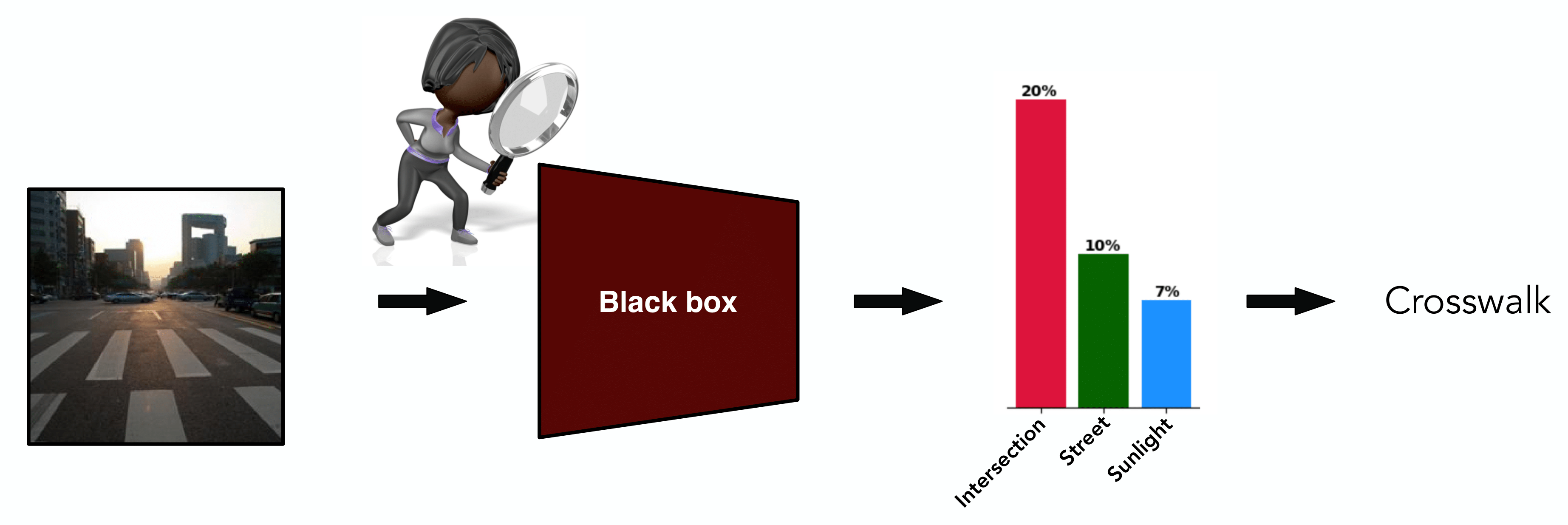
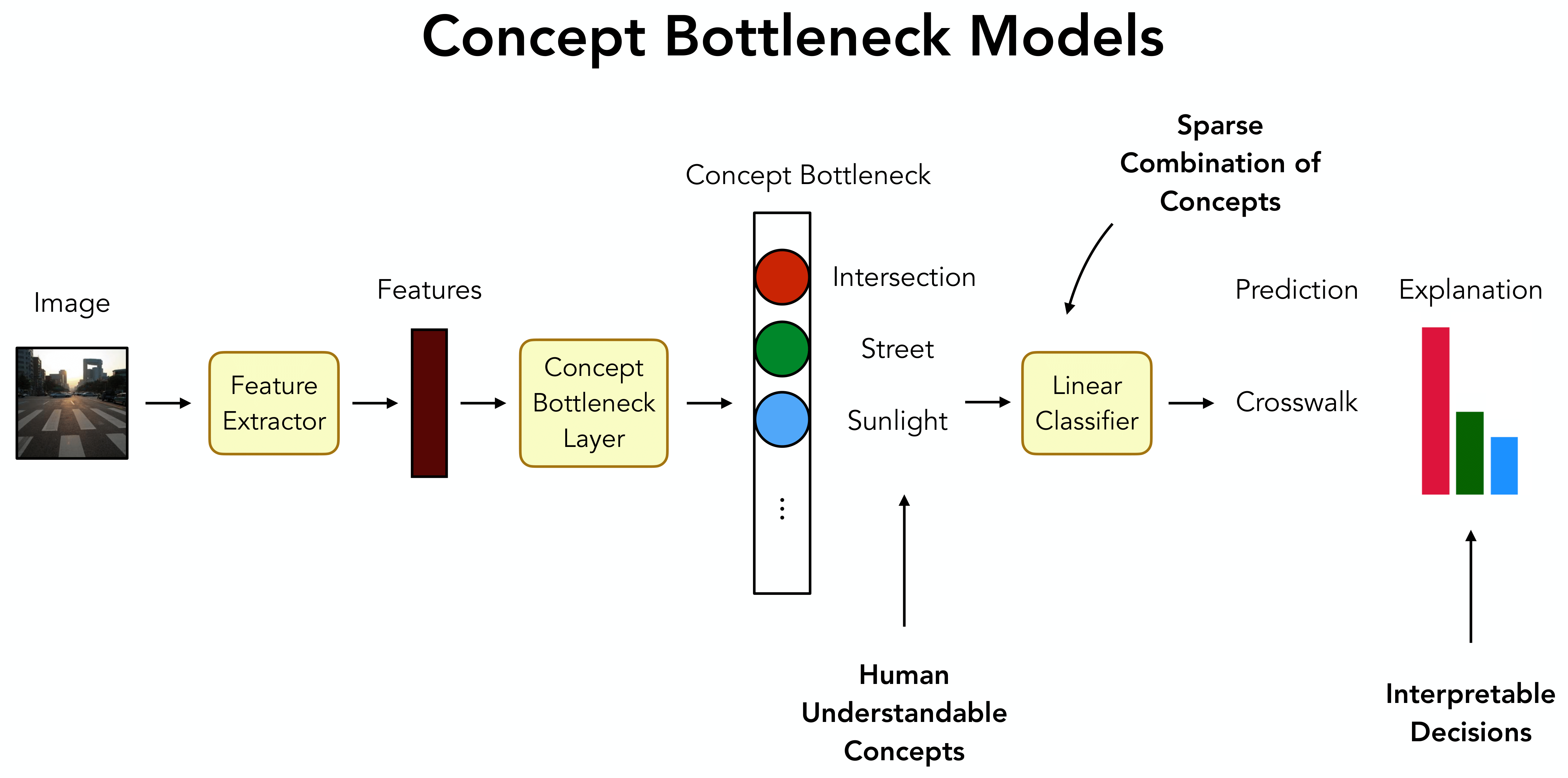
Deep neural networks are powerful but lack transparency, posing risks in safety-critical applications. Concept Bottleneck Models (CBMs^{1 2 3}) are a type of framework which enhances model interpretability by making model decisions transparent. These models map the image features of a neural network to a set of human understandable concepts, which are then typically combined in a linear classifier to give the model prediction.

CLIP (Contrastive Language-Image Pretraining)

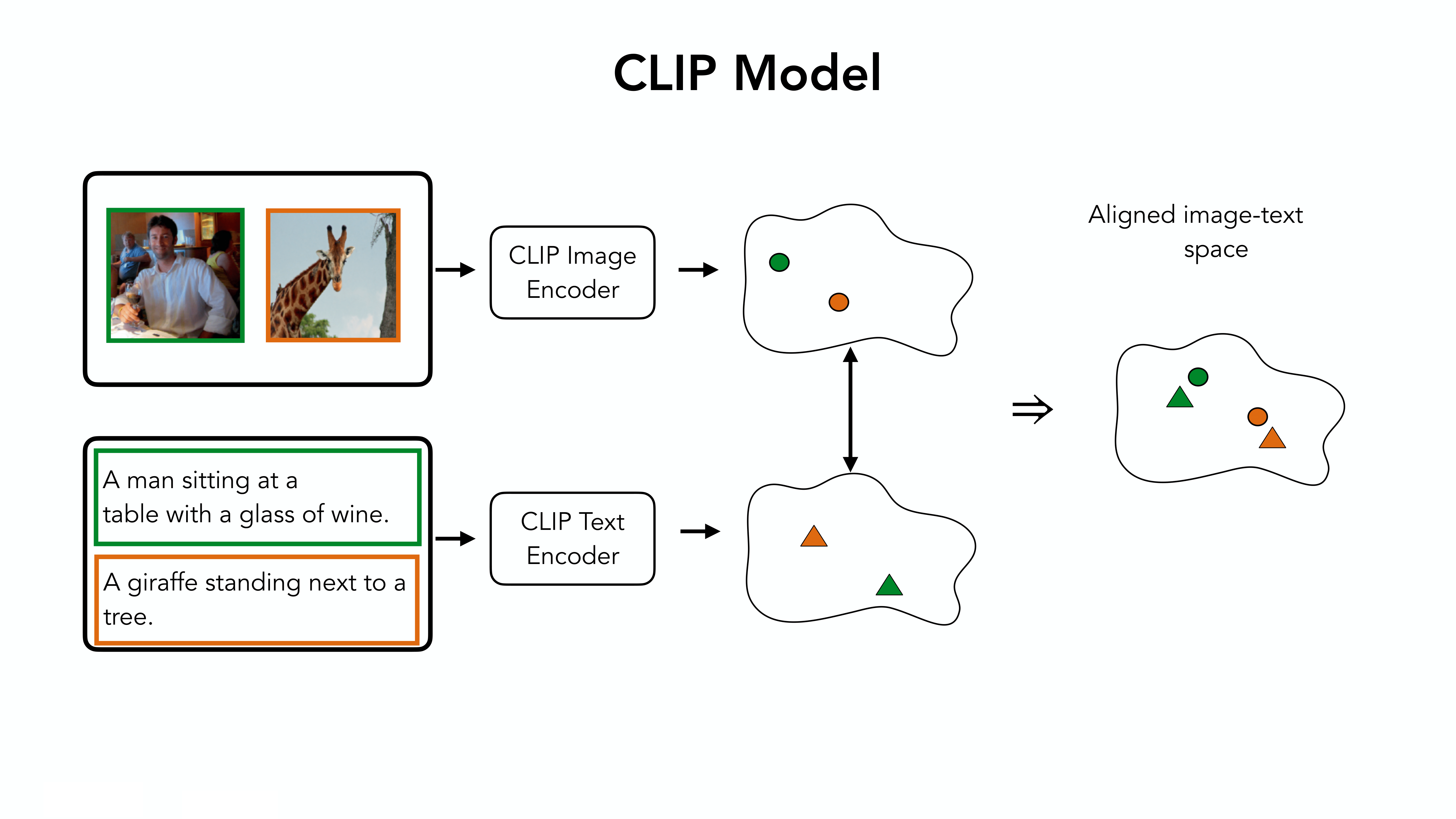
In this work, we use the CBM framework to probe the concepts learned by CLIP and furthermore, express the CLIP predictions as a combination of human understandable concepts. CLIP (Contrastive Language-Image Pretraining) models use paired image and text to learn a vision-language aligned space by pulling together corresponding image-text pairs and pushing away other image-text pairs.

Overview of the Method

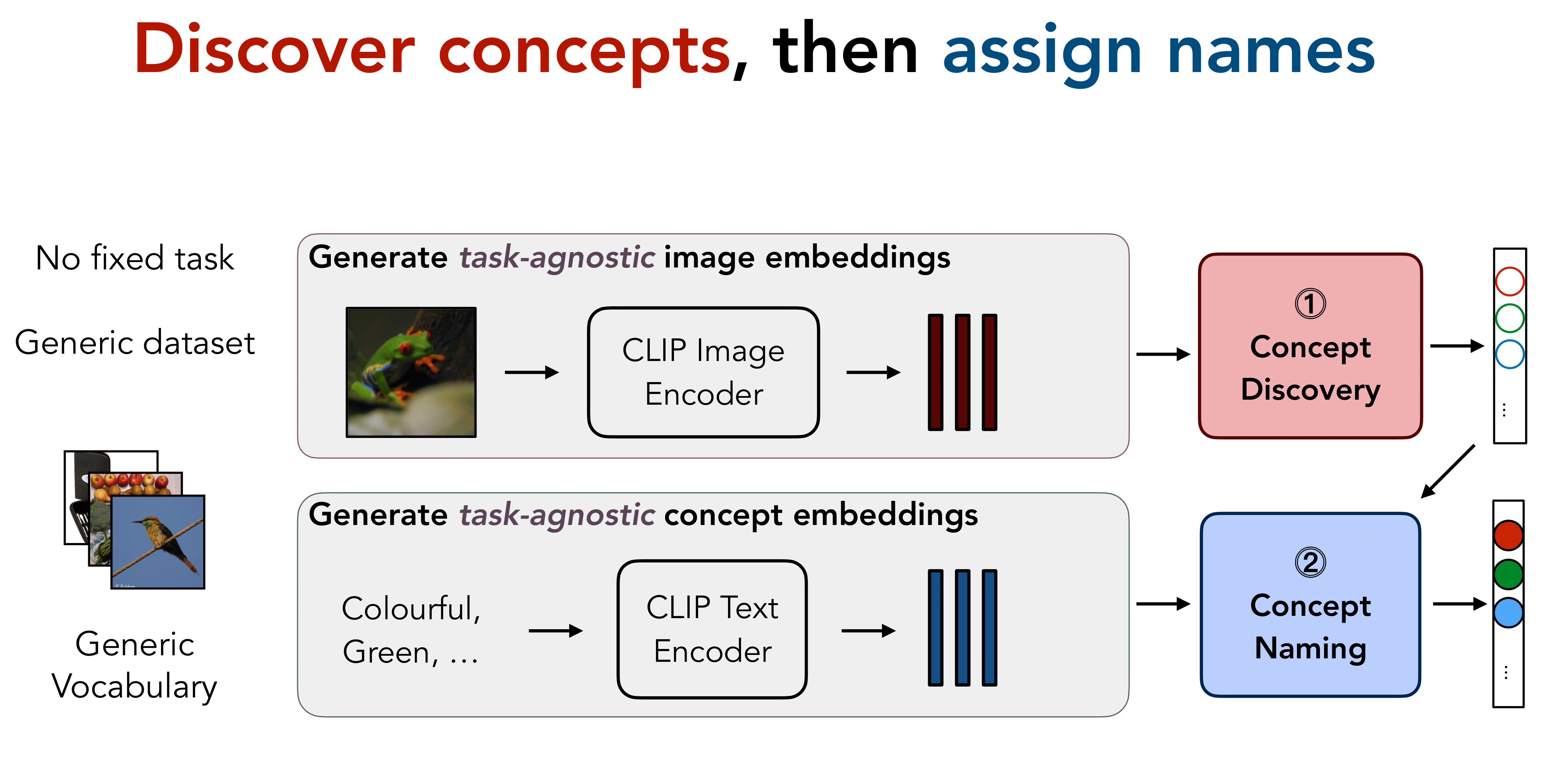
Figure 3 shows an overview of our method. Unlike earlier approaches, we propose to train a task-agnostic concept discovery module to discover the learned concepts which can be used for multiple downstream datasets. Moreover, the use of a generic vocabulary for naming the discovered concepts makes our approach task-agnostic in contrast to previous works, which use LLMs to get task-relevant concept names and align the model to these predefined set of concepts.

Concept Discovery

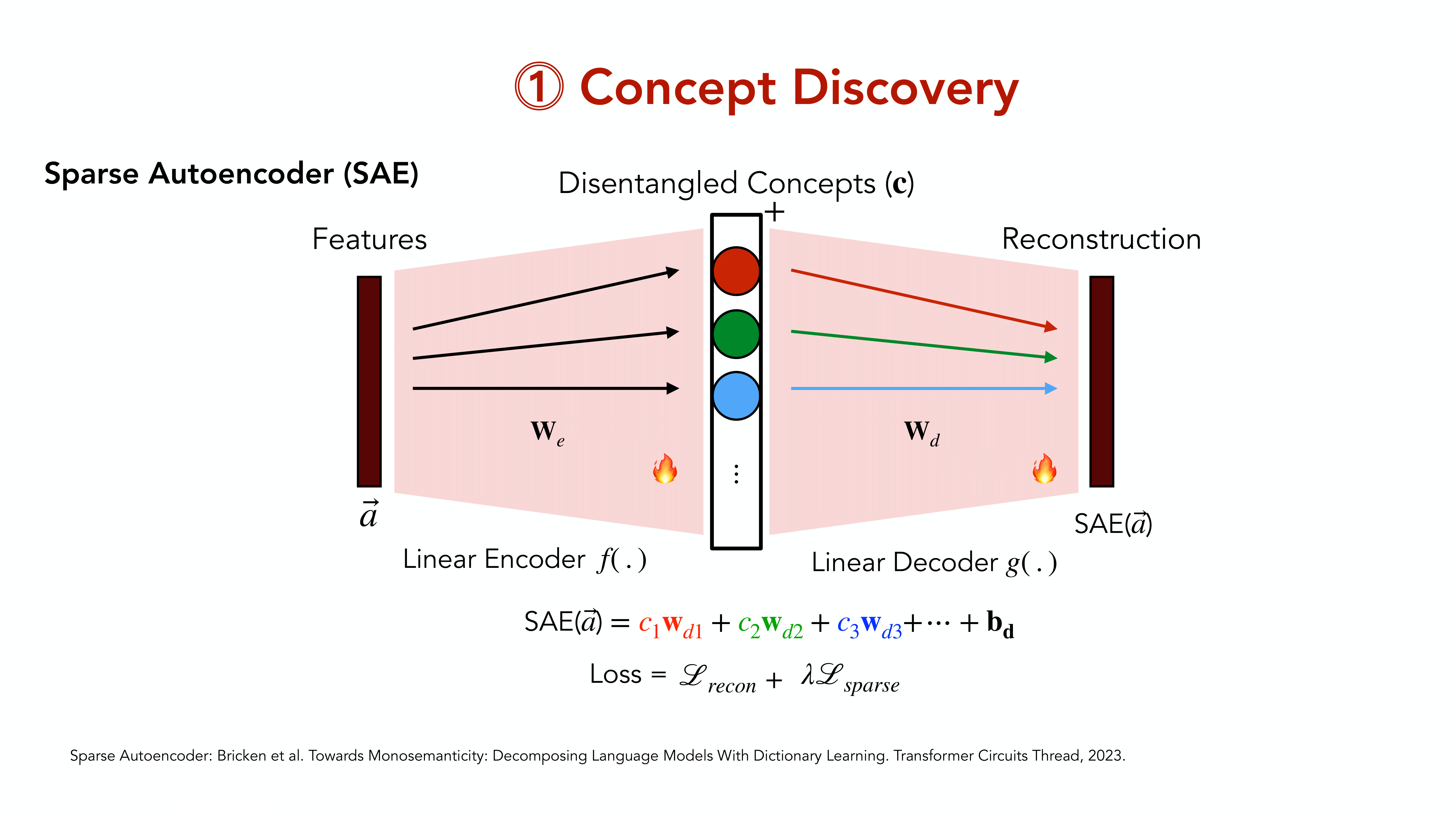
To discover the concepts learned by the model, we adapt the sparse autoencoder (SAE) approach as described by ⁴.

The Sparse Autoencoders (SAEs) proposed by ⁴ consist of a linear encoder \(f(\cdot)\) with weights \(\vec W_{E}\in\mathbb R^{d\times h}\), a ReLU non-linearity \(\phi\), and a linear decoder \(g(\cdot)\) with weights \(\vec W_D\in\mathbb R^{h\times d}\). For a given input \(\vec a\), the SAE computes:

\[ \begin{align} \text{SAE}(\vec a) = (g \circ \phi \circ f) (\vec a) = \vec W_D^T\;\phi\left(\vec W_E^T \vec a\right)\;. \end{align} \]

Importantly, the hidden representation \(f(\vec a)\) is of significantly higher dimensionality than the CLIP embedding space (i.e., \(h\gg d\)), but optimised to activate only very sparsely. Specifically, the SAE is trained with an \(L_2\) reconstruction loss, as well as an \(L_1\) sparsity regularisation:

\[ \begin{align} \mathcal L_\text{SAE}(\vec a) = \lVert\text{SAE}(\vec a) - \vec a\rVert^2_2 + \lambda_1 \lVert \phi(f(\vec a))\rVert_1 \end{align} \]

with \(\lambda_1\) a hyperparameter. To discover a diverse set of concepts for usage in downstream tasks, we train the SAE on a large dataset \(\mathcal{D}_\text{extract}\); given the reconstruction objective, no labels for this dataset are required.

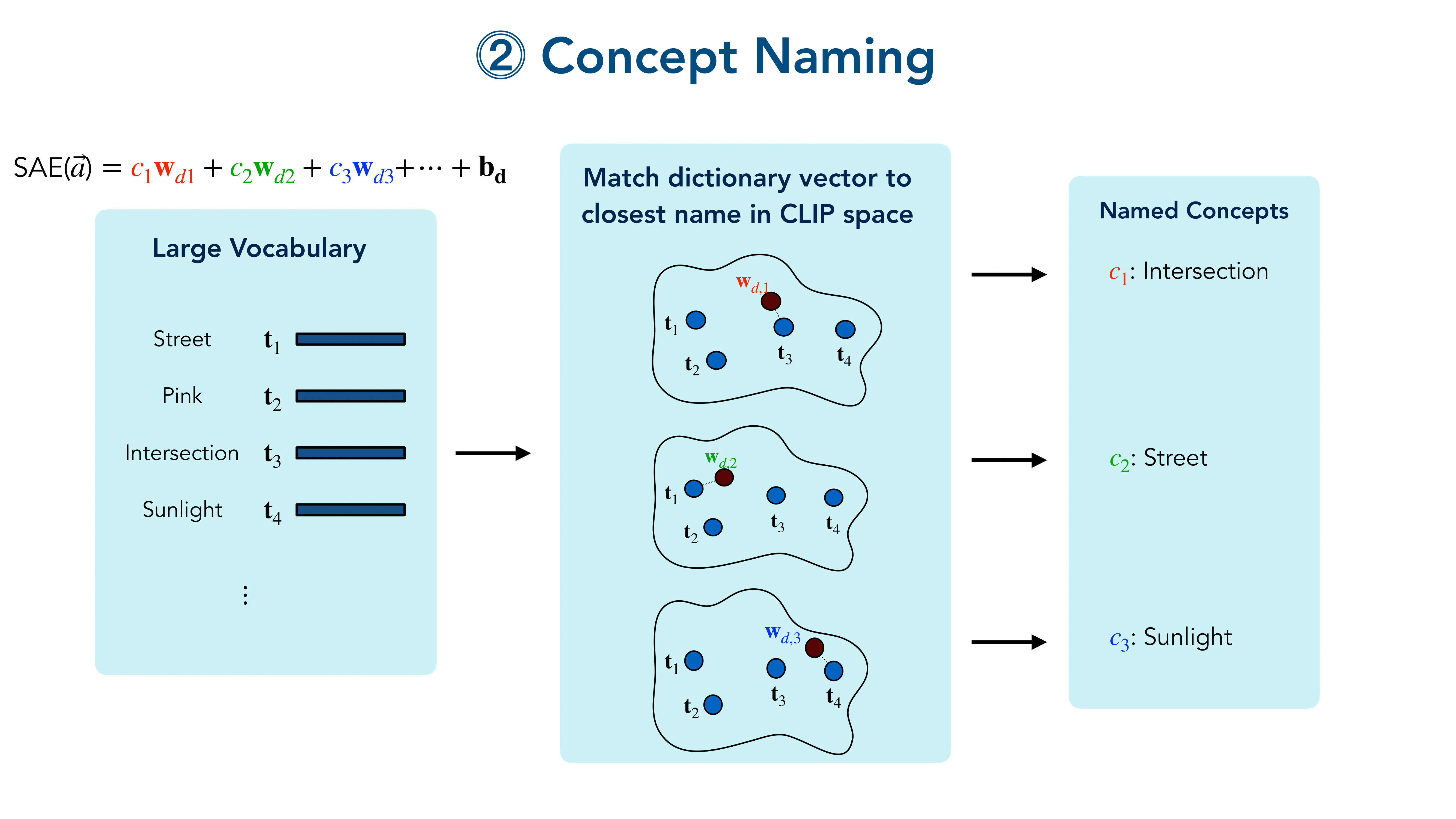
Automated Concept Naming

Once we trained the SAE, we automatically name the individual feature dimensions in the hidden representation of the SAE. For this, we use a large vocabulary \(\mathcal{V}=\{v_1,v_2,\dots\}\) of English words, which we embed via the CLIP text encoder \(\mathcal T\) to obtain word embeddings \(\mathcal E=\{\vec e_1, \vec e_2, \dots\}\).

To name the SAE’s hidden features, we propose to leverage the fact that each of the SAE neurons \(c\) is assigned a specific dictionary vector \(\vec p_c\), corresponding to a column of the decoder weight matrix:

\[ \begin{align} \vec p_c = [\vec W_D]_c \in \mathbb R^{d}\;. \end{align} \]

If the SAE indeed succeeds to decompose image representations given by CLIP into individual concepts, we expect the \(\vec p_c\) to resemble the embeddings of particular words that CLIP has learnt to expect in a corresponding image caption.

Hence, to name the ‘concept’ neuron \(c\) of the SAE, we propose to assign it the word \(s_c\) of the closest text embedding in \(\mathcal E\):

\[ \begin{equation} s_c = \arg\min_{v \in \mathcal{V}} \;\left[\cos\left(\vec p_c,\mathcal{T}(v)\right) \right]\;. \end{equation} \]

Note that this setting is equivalent to using the SAE to reconstruct a CLIP feature when only the concept to be named is present. As CLIP was trained to optimise cosine similarities between text and image embeddings, using the cosine similarity to assign names to concept nodes is a natural choice in this context.

Constructing Concept Bottleneck Models

Thus far, we trained an SAE to obtain sparse representations, and named individual ’neurons’ by leveraging the similarity between dictionary vectors \(\vec p_c\) to word embeddings obtained via CLIP’s text encoder \(\mathcal T\).

Such a sparse decomposition into named ‘concepts’ constitutes the ideal starting point for constructing interpretable CBMs for a given labelled dataset \(\mathcal D_\text{probe}\), we can now train a linear transformation \(h(\cdot)\) on the SAE’s sparse concept activations, yielding our CBM \(t(\cdot)\):

\[ \begin{align} t(\vec x_i) = (\underbrace{h}_\text{Probe} \circ \;\underbrace{\phi \circ f}_\text{SAE} \; \circ \underbrace{\mathcal I}_\text{CLIP}) (\vec x_i)\;. \end{align} \]

Here, \(\vec x_i\) denotes an image from the probe dataset. The probe is trained using the cross-entropy loss, and to increase the interpretability of the resulting CBM classifier, we additionally apply a sparsity loss to the probe weights:

\[ \begin{align} \mathcal L_\text{probe}(\vec x_i) = \text{CE}\left(t(\vec x_i), y_i\right)+ \lambda_2 \lVert\omega\rVert_1 \end{align} \]

where, \(\lambda_2\) is a hyperparameter, \(y_i\) the ground truth label of \(\vec x_i\) in the probe dataset, and \(\omega\) denotes the parameters of the linear probe.

Evaluations

Here, we showcase some of the discovered concepts and the assigned names of our approach.

Task-Agnosticity and Accuracy of Concepts

Figure 7 visualizes the top activating images across four datasets for various concepts that were discovered and named as described above.

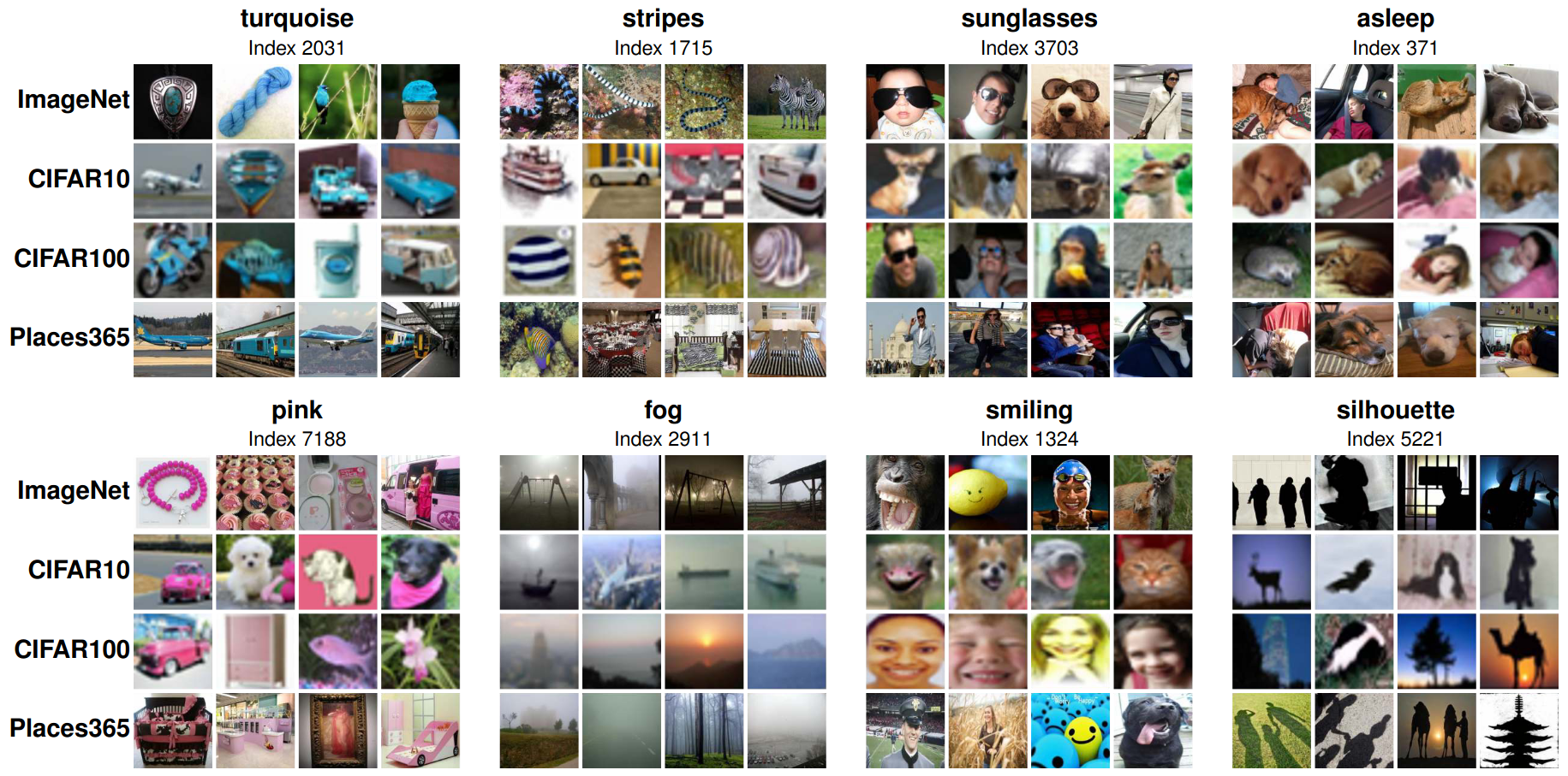
In particular, we show examples for various low-level concepts (turquoise, pink, striped), object and scene-specific concepts (sunglasses, fog, silhouette), as well as higher-level concepts (asleep, smiling), and find that the visualized concepts not only exhibit a high level of semantic consistency, but also that the automatically chosen names for the concepts accurately reflect the common feature in the images, despite coming from very different datasets. This highlights the promise of the SAE for disentangling representations into human interpretable concepts as well as of the proposed strategy for naming those concepts.

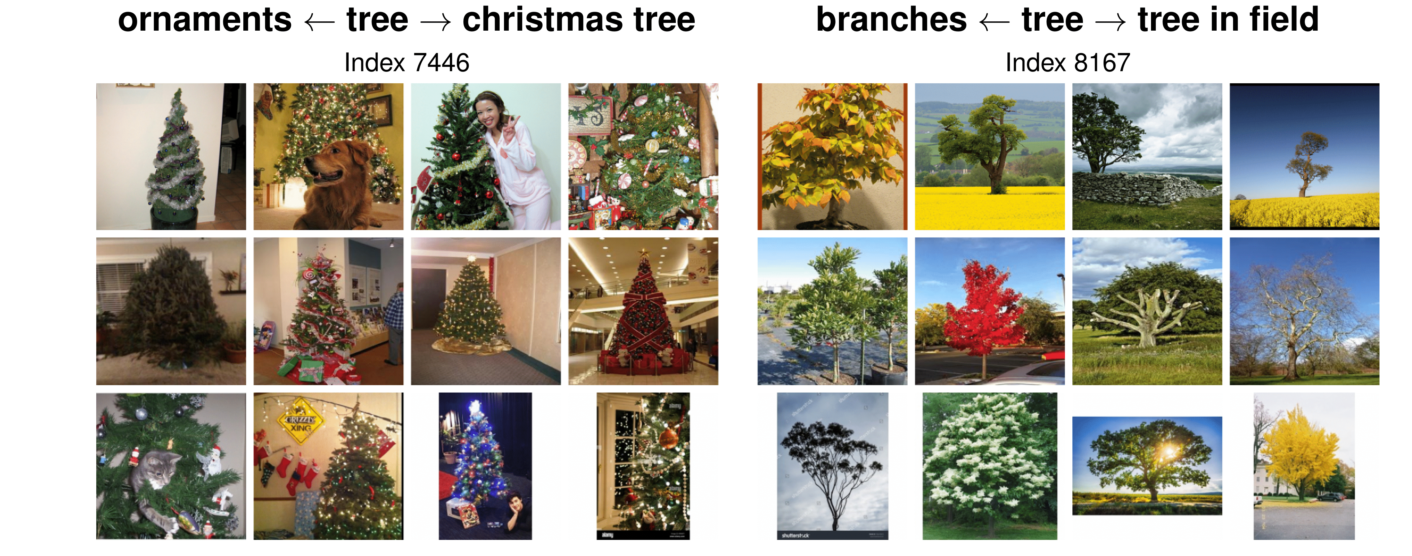
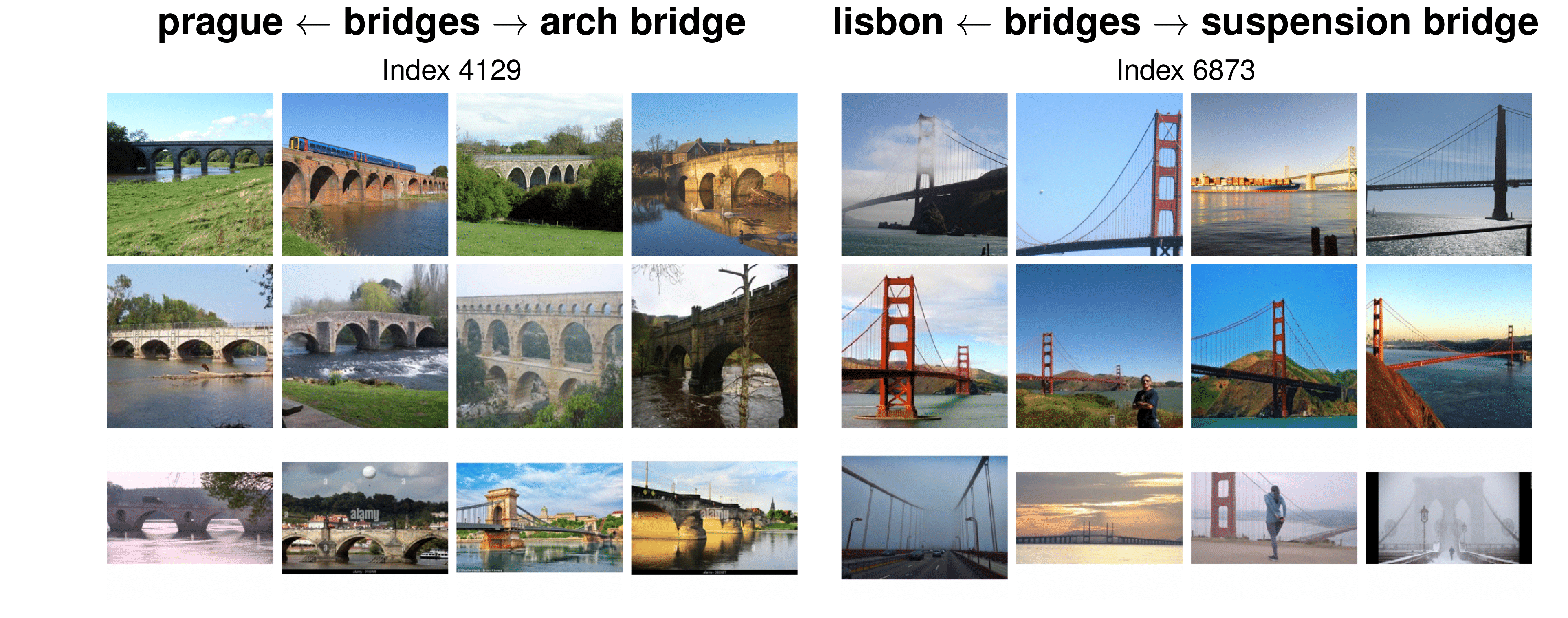
Impact of Vocabulary on Concept Name Granularity

To explore the impact of vocabulary on concept naming, Figure 8 visualizes examples of concept pairs that are originally assigned the same name (e.g., bottom: ‘bridges’), but visually correspond to distinct modalities of the concept. We find that we can improve the granularity of the assigned concept by adding more fine-grained names to the vocabulary \(\mathcal{V}\) (e.g. ‘arch bridge’, ‘suspension bridge’). Conversely, removing the assigned name ‘bridge’ from the vocabulary leads to worse name assignments (e.g. ‘prague’, ’lisbon’; interestingly, note that the cities contain a prominent arch and suspension bridge, respectively). This suggests that the granularity and size of the vocabulary can significantly affect the name accuracy, and can also serve as a tool for practitioners to control the granularity of assigned names depending on the use case.

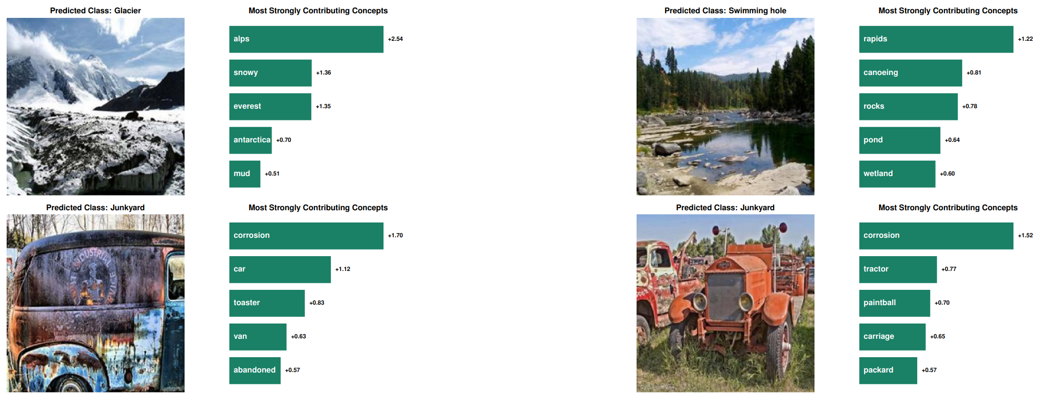
Local Explanations (Image-Level)

Figure 9 shows qualitative examples of local explanations from our DN-CBM, i.e., explanations of individual decisions. For each image, we show the most contributing concepts along with their contribution strengths. We find that the used concepts are intuitive and class-relevant, aiding interpretability. They are also diverse and include objects in the scenes (e.g., ‘rocks’ for ‘swimming hole’, top-right), similar features (e.g., ’toaster’ given the corroded surface for ‘junkyard’, bottom-left), and high-level concepts (e.g., ‘abandoned’ for ‘junkyard’, bottom-left). Interestingly, we also find concepts associated with the class (e.g., ‘alps’ or ’everest’ for ‘glacier’, top-left), which shows that the model’s decision is also based on what a scene looks like, akin to ProtoPNets.⁵ Finally, we observe that the concepts for predicting the same class change based on the contents of the image, e.g., in the bottom row, we find that despite both images depicting a junkyard where the most influential concept is ‘corrosion’, the second highest concepts are ‘car’ and ’tractor’ respectively, reflecting the image contents.

Conclusion

In this work, we proposed Discover-then-Name CBM (DN-CBM), a novel CBM approach that uses sparse autoencoders to discover and automatically name concepts learnt by CLIP, and then use the learnt concept representations as a concept bottleneck and train linear layers for classification. We find that this simple approach is surprisingly effective at yielding semantically consistent concepts with appropriate names. Further, we find despite being task-agnostic, i.e. only extracting and naming concepts once, our approach can yield performant and interpretable CBMs across a variety of downstream datasets. Our results further corroborate the promise of sparse autoencoders for concept discovery. Training a more ‘foundational’ sparse autoencoder with a much larger dataset (e.g. at CLIP scale) and concept space dimensionality (with hundreds of thousands or millions of concepts) to obtain even more general-purpose CBMs, particularly for fine-grained classification, would be a fruitful area for future research.

References