Tree-Ensemble Repair through Constrained Optimization
Written by Chaahat Jain
Published on 4th November 2026
Paper: arXiv, NeurIPS'26 | Software: GitHub | Keywords: model repair, constrained optimization, fairness, safety
When accuracy is not enough
Meet Alex. He trains AI models for a delivery service. One model decides which orders qualify for priority delivery; another controls a delivery robot. Both perform well on the test data. But Alex also has requirements that accuracy alone does not capture.
For the priority model, changing a customer’s gender while keeping every other input identical should not change the decision. This is the flavor of fairness we study: two inputs that differ only in a protected attribute must receive the same label.1
For the robot, completing most deliveries is not enough. It must also avoid actions that lead to a situation where failure becomes unavoidable. Accelerating towards an obstacle can be unsafe long before a collision happens. Safety, in our setting, means staying in the region where failure can still be avoided, whatever the outcome of the chosen action.
Alex does not want to start over. He wants to fix the unacceptable decisions while keeping as much of his models’ performance as possible. Figure 1 shows our approach: find violations, repair the model’s leaf scores, add a tree when needed, and check again. The requirement is the only part that changes between fairness and safety.
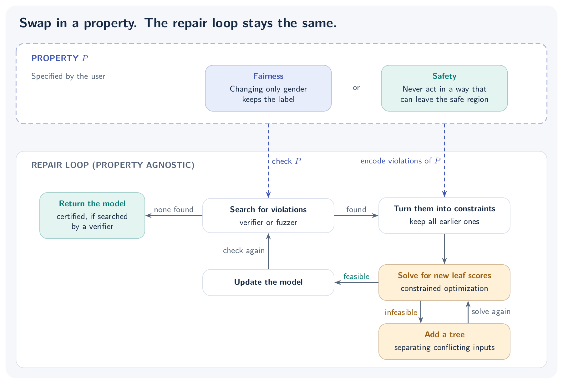
One view of fairness and safety
Fairness and safety sound like different problems, but both answer the same question: which combinations of inputs and predictions are allowed? Fairness looks at two inputs at once; safety looks at one.
Let $\mathcal{X}$ be the input space, $\mathcal{Y}$ the finite set of labels, and $f$ the model. A property
$$ P:\mathcal{X}^{k}\times\mathcal{Y}^{k}\longrightarrow\{0,1\} $$takes $k$ inputs together with their predicted labels and says whether that combination is acceptable. The model satisfies $P$ if $P\bigl(\mathbf{x},f(\mathbf{x})\bigr)=1$ for every tuple of inputs $\mathbf{x}$. In formal methods, such properties over several inputs are called hyperproperties.2
Both of Alex’s requirements fit this form. Let $p$ be the protected attribute, $\mathcal{X}^{S}$ the states from which failure can still be avoided, and $\mathcal{Y}^{U}(x)$ the unsafe actions in state $x$:
$$ \begin{aligned} \text{Fairness:}&\quad \Bigl(\textstyle\bigwedge_{j\ne p}x_j=x'_j\Bigr)\Longrightarrow f(x)=f(x'),\\[3pt] \text{Safety:}&\quad x\in\mathcal{X}^{S}\Longrightarrow f(x)\notin\mathcal{Y}^{U}(x). \end{aligned} $$An action is unsafe if any of its possible outcomes leaves the safe region.3 Because the safe region already accounts for what can happen later, a rule about a single state and action is enough.
Our method works for any property of this form, as long as each violation involves finitely many inputs and some classifier can satisfy the property. Only the top panel of Figure 1 changes.
From counterexamples to repair constraints
A counterexample shows exactly where the model breaks a requirement. A verifier such as Veritas 4 searches for counterexamples exhaustively; if it finds none, the property is proven. This can be very slow, so testing techniques such as fuzzing offer a cheaper alternative: they find violations quickly but cannot prove that none remain.
Formally, a counterexample is a tuple $\mathbf{e}$ with $P\bigl(\mathbf{e},f(\mathbf{e})\bigr)=0$. We turn it into a repair formula $\varphi_P(\mathbf{e})$ stating which labels the repaired model $f'$ may assign to it:
$$ \begin{aligned} \varphi_{\mathrm{fair}}(e_1,e_2) &=\bigl[f'(e_1)=f'(e_2)\bigr],\\[3pt] \varphi_{\mathrm{safe}}(e) &=\bigwedge_{y\in\mathcal{Y}^{U}(e)} \neg\bigl[f'(e)=y\bigr]. \end{aligned} $$A counterexample rarely dictates a single correct answer. The customer pair could both become “yes” or both “no”; the robot may have several safe actions. Repair formulae keep this freedom and let the optimizer choose. Such a formula exists for any property, because a fixed tuple of inputs has only finitely many label combinations.
As the loop runs, we collect counterexamples in a set $E$ and require all their repair formulae to hold at once. We only encode what is acceptable on these inputs, never the property over the whole input space.
Why tree ensembles?
A decision tree is a sequence of questions. Is the package heavy? Is the destination nearby? Is the robot moving fast? An input follows one path through each tree to a leaf. Each leaf stores a score per label; the ensemble adds up the scores of the reached leaves and predicts the label with the highest total:
$$ S_y(x)=\sum_{\ell\in\operatorname{OC}(x)}\nu_{\ell,y}, \qquad f(x)=\operatorname*{arg\,max}_{y\in\mathcal{Y}}S_y(x). $$Here $\nu_{\ell,y}$ is leaf $\ell$’s score for label $y$, and $\operatorname{OC}(x)$, the input’s output configuration 5, is the set of leaves it reaches, one per tree. We therefore know exactly which parameters decide each prediction.
Imagine an unsafe robot state where the scores are 2.4 for “accelerate” and 2.1 for “brake.” As Figure 2 shows, adjusting the reached leaves so that braking wins fixes this decision without rebuilding any tree. Leaves that no counterexample reaches stay untouched.
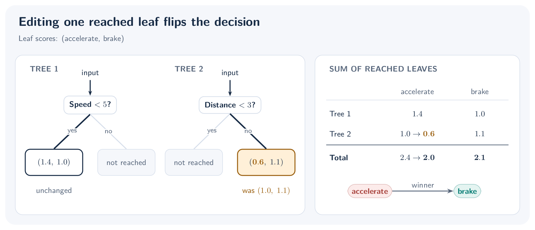
Repair is therefore local. It can also generalize: other inputs that share the adjusted leaves may be fixed along the way.
Repair as an optimization problem
We choose the new leaf scores $\nu'$ by solving a mixed-integer linear program (MILP) with two goals:
- Fix the counterexamples. These are hard constraints.
- Change the model as little as possible. This is the objective.
Only the leaves reached by some counterexample, $L_E$, may change. For each counterexample input $e_i$ and label $y$, a binary variable $z_{i,y}$ is 1 exactly when $y$ has the highest score for $e_i$; standard big-$M$ constraints link it to the leaf scores.6 Repair formulae then become simple linear constraints:
| Requirement | Linear constraint |
|---|---|
| Assign label $y$ to $e_i$ | $z_{i,y}=1$ |
| Make $e_i$ and $e_j$ agree | $z_{i,y}=z_{j,y}$ for every $y$ |
| Forbid an unsafe action $y$ at $e_i$ | $z_{i,y}=0$ |
Combinations of these using AND, OR, and NOT can be encoded with standard techniques.6
The objective keeps the repaired model close to the original:
$$ \min_{\nu',s}\quad \underbrace{\sum_{(x,y)\in D'}s_x}_{\text{penalize disrupted predictions}} + \lambda\, \underbrace{\sum_{\ell\in L_E}\sum_{c\in\mathcal{Y}} \left|\nu'_{\ell,c}-\nu_{\ell,c}\right|}_{\text{keep leaf changes small}}. $$Here $D'$ contains the training examples the model currently classifies correctly, and $s_x$ measures by how much a wrong label outscores the correct one (zero if the prediction stays correct). Every solution satisfies all repair constraints; the objective picks the one that best preserves accuracy, though it cannot guarantee it.
When repair is infeasible
Sometimes no choice of leaf scores satisfies all constraints. The MILP is then infeasible, and more solver time will not help.
Scenario 1: two inputs need different labels but reach exactly the same leaves, so they always receive the same scores.
Scenario 2: the inputs reach different leaves, but the trees cannot combine their features correctly. Consider a robot at a junction that must turn left or right. It faces north or south, and an obstacle blocks either the east or the west exit. The safe action is to turn towards the open exit. The controller in Figure 3 has two trees with one split each: Tree 1 asks whether the robot faces north, Tree 2 whether the obstacle is to the east. Every leaf stores scores as (turn left, turn right).
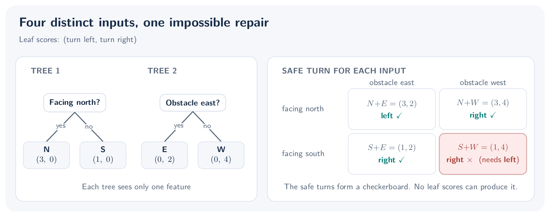
A robot facing north with the obstacle to the east reaches leaves $N$ and $E$: $(3,0)+(0,2)=(3,2)$, so it correctly turns left. A robot facing south with the obstacle to the west reaches $S$ and $W$: $(1,0)+(0,4)=(1,4)$, so it turns right, into the blocked exit. It should turn left.
Raising the left-turn score at $S$ would fix this, but the south/east input also uses $S$ and must turn right. Even adjusting all four leaves cannot make every decision safe. The correct turn depends on heading and obstacle together, while each tree sees only one of them.
Adding the missing distinction
When repair is infeasible, the solver identifies a minimal set of conflicting constraints 7: removing any one of them resolves the conflict. We train a new tree that sends the corresponding inputs to separate leaves. Its leaves start at zero, so predictions do not change until we solve again, now with extra scores that can treat those inputs separately. For a finite set of counterexamples and a satisfiable property, repeating this always restores feasibility.
Check again
Changing a leaf score affects every input that reaches that leaf. This can fix violations we have not seen yet, but it can also break decisions that were correct. Alex therefore checks the repaired model again and repeats the loop in Figure 1. All earlier constraints are kept, so a fixed violation cannot return. Once a verifier finds no more counterexamples, the property is certified.
Experiments
Fairness: all 50 models verified
We evaluated fairness on ten standard datasets with five folds each, giving 50 XGBoost models.8 To make full verification tractable, we first compressed them with LOP 9, at a small cost in validation performance.
| Model | Verified fair |
|---|---|
| Compressed XGBoost (LOP) | 14 / 50 |
| MILP repair | 50 / 50 |
| FATT 10 | 30 / 50 |
| BuDRO 11 | 42 / 50 |
After repair, every model was verified fair, and none needed an extra tree. The median repair took 30 seconds, although hard instances took considerably longer.
The accuracy cost was small (Figure 4). Balanced accuracy, which weights each class equally, dropped by about 1.7 percentage points relative to the original XGBoost models: 0.3 from compression and 1.4 from repair. The fairness-aware training methods FATT and BuDRO lost about 9 and 4 points.
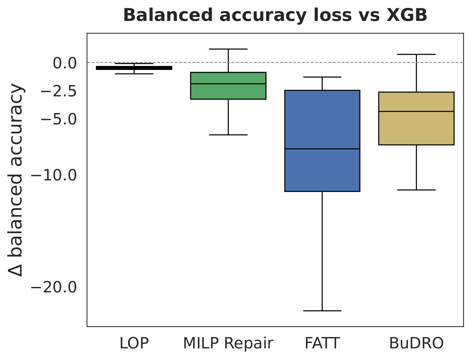
Safety: better behavior on unseen initial states
For safety, we used planning and control tasks such as package transport, car following, and pole balancing from the benchmark suite of 12. Tree ensembles were trained to imitate existing neural policies. 31 of the 38 benchmarks needed repair.
Exhaustive verification is too expensive here, so we found counterexamples with the fuzzer from 12. We repaired using runs from 5,000 initial states and evaluated on 5,000 different ones, to test whether repairs carry over to new situations. We report two metrics: %Safe, the fraction of initial states from which the policy avoids failure under all outcomes, and %Goal, the fraction of runs that reach the goal.
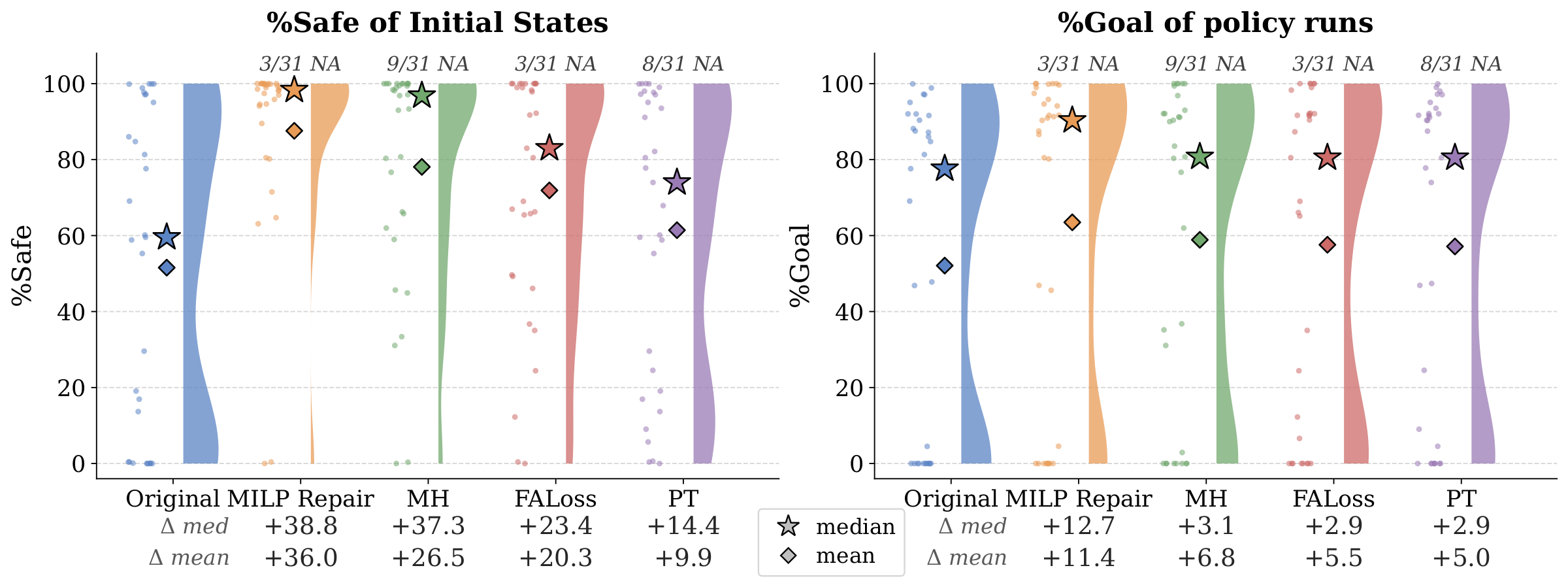
Safer policies also reached their goal more often. The loop finished on 28 of the 31 benchmarks, 22 of them within ten minutes; the other three hit time or memory limits, and we report their last policy. Only two benchmarks needed extra trees.
What this gives Alex
A concrete debugging loop: state the requirement, find counterexamples, repair the responsible leaf scores, and check again. When the trees cannot express the required behavior, a targeted extra tree gives the repair room to work. In our experiments, this gave verified fairness at a small accuracy cost and large gains in safety.
References
-
S. Calzavara, L. Cazzaro, C. Lucchese, and F. Marcuzzi. Explainable Global Fairness Verification of Tree-Based Classifiers. SaTML, 2023. ↩︎
-
M. R. Clarkson and F. B. Schneider. Hyperproperties. Journal of Computer Security, 18(6):1157–1210, 2010. ↩︎
-
C. Jain, L. Cascioli, L. Devos, M. Vinzent, M. Steinmetz, J. Davis, and J. Hoffmann. Safety Verification of Tree-Ensemble Policies via Predicate Abstraction. ECAI, 2024. ↩︎
-
L. Devos, W. Meert, and J. Davis. Versatile Verification of Tree Ensembles. ICML, 2021. ↩︎
-
L. Devos, L. Perini, W. Meert, and J. Davis. Detecting Evasion Attacks in Deployed Tree Ensembles. ECML PKDD, 2023. ↩︎
-
J. P. Vielma. Mixed Integer Linear Programming Formulation Techniques. SIAM Review, 2015. ↩︎ ↩︎
-
J. Gleeson and J. Ryan. Identifying Minimally Infeasible Subsystems of Inequalities. INFORMS Journal of Computing, 1990. ↩︎
-
T. Chen and C. Guestrin. XGBoost: A Scalable Tree Boosting System. KDD, 2016. ↩︎
-
L. Devos, T. Martens, D. C. Oruc, W. Meert, H. Blockeel, and J. Davis. Compressing Tree Ensembles through Level-Wise Optimization and Pruning. ICML, 2025. ↩︎
-
F. Ranzato, C. Urban, and M. Zanella. Fairness-Aware Training of Decision Trees by Abstract Interpretation. CIKM, 2021. ↩︎
-
A. Vargo, F. Zhang, M. Yurochkin, and Y. Sun. Individually Fair Gradient Boosting. ICLR, 2021. ↩︎
-
C. Jain, D. Sherbakov, M. Vinzent, M. Steinmetz, J. Davis, and J. Hoffmann. Policy Safety Testing in Non-Deterministic Planning: Fuzzing, Test Oracles, Fault Analysis. ECAI, 2025. ↩︎ ↩︎